Algorithms

Scientific documentation of the algorithms used in ESPectre for Wi-Fi CSI-based motion detection.

Table of Contents

• Overview
• Processing Pipeline
• Gain Lock (Hardware Stabilization)
• CV Normalization (Gain-Invariant Turbulence)
• Subcarrier Selection (NBVI)
• Signal Conditioning
• MVS: Moving Variance Segmentation
• ML: Neural Network Detector
• References

Overview

ESPectre uses a combination of signal processing algorithms to detect motion from Wi-Fi Channel State Information (CSI).

Processing Pipeline

┌───────────────────────────────────────────────────────────────────────────────────┐
│                           CSI PROCESSING PIPELINE                                  │
├───────────────────────────────────────────────────────────────────────────────────┤
│                                                                                   │
│  ┌──────────┐    ┌──────────┐    ┌──────────────┐    ┌─────────────┐              │
│  │ CSI Data │───▶│Gain Lock │───▶│ Band Select  │───▶│ Turbulence  │              │
│  │ N subcs  │    │ AGC/FFT  │    │ 12 subcs     │    │ σ/μ (CV)    │              │
│  └──────────┘    └──────────┘    └──────────────┘    └──────┬──────┘              │
│                  (3s, 300 pkt)   (7.5s, 10×window)          │                     │
│                                                             ▼                     │
│  ┌───────────┐    ┌───────────────┐    ┌─────────────────┐  ┌──────────────────┐  │
│  │ IDLE or   │◀───│ Adaptive      │◀───│ Moving Variance │◀─│ Optional Filters │  │
│  │ MOTION    │    │ Threshold     │    │ (window=75)     │  │ LowPass + Hampel │  │
│  └───────────┘    └───────────────┘    └─────────────────┘  └──────────────────┘  │
│                                                                                   │
└───────────────────────────────────────────────────────────────────────────────────┘

Calibration sequence (at boot): 1. Gain Lock (3s, 300 packets): Collect AGC/FFT, lock values 2. Band Calibration (~7.5s, 10 × window_size packets): Select 12 optimal subcarriers, calculate baseline variance

With default window_size=75, this means 750 packets. If you change segmentation_window_size, the calibration buffer adjusts automatically.

Data flow per packet (after calibration): 1. CSI Data: Raw I/Q values for 64 subcarriers (HT20 mode) - Espressif format: [Q₀, I₀, Q₁, I₁, ...] (Imaginary first, Real second per subcarrier) 2. Amplitude Extraction: |H| = √(I² + Q²) for selected 12 subcarriers 3. Spatial Turbulence (CV): CV = σ(amplitudes) / μ(amplitudes) - gain-invariant variability 4. Hampel Filter (optional): Remove outliers using MAD 5. Low-Pass Filter (optional): Remove high-frequency noise (Butterworth 1st order) 6. Moving Variance: Var(turbulence) over sliding window 7. Adaptive Threshold: Compare variance to Pxx(baseline_mv) → IDLE or MOTION

Gain Lock (Hardware Stabilization)

The Problem

The ESP32 WiFi hardware includes automatic gain control (AGC) that dynamically adjusts signal amplification based on received signal strength. While this improves data decoding reliability, it creates a problem for CSI sensing:

How It Works

Gain Lock stabilizes CSI amplitude measurements by locking the ESP32's AGC and FFT scaling. Based on Espressif's esp-csi recommendations.

The lock happens in a dedicated phase BEFORE band calibration to ensure clean data:

┌──────────────────────────────────────────────────────────────────────┐
│                    TWO-PHASE CALIBRATION                              │
├──────────────────────────────────────────────────────────────────────┤
│                                                                      │
│  PHASE 1: GAIN LOCK (~3 seconds, 300 packets)                        │
│  ┌─────────────┐    ┌─────────────┐    ┌─────────────┐              │
│  │  Read PHY   │───▶│   Collect   │───▶│  Calculate  │              │
│  │  agc_gain   │    │  agc_samples│    │   Median    │              │
│  │  fft_gain   │    │  fft_samples│    │             │              │
│  └─────────────┘    └─────────────┘    └──────┬──────┘              │
│                                               │                      │
│  Packet 300:                                  ▼                      │
│  ┌──────────────────────────────────────────────────────────────┐   │
│  │  phy_fft_scale_force(true, median_fft)                       │   │
│  │  phy_force_rx_gain(true, median_agc)                         │   │
│  │  → AGC/FFT now LOCKED                                        │   │
│  └──────────────────────────────────────────────────────────────┘   │
│                           │                                          │
│                           ▼                                          │
│  PHASE 2: BAND CALIBRATION (~7.5 seconds, 10 × window_size packets) │
│  ┌──────────────────────────────────────────────────────────────┐   │
│  │  Now all packets have stable gain!                           │   │
│  │  → Baseline variance calculated on clean data                │   │
│  │  → Subcarrier selection more accurate                        │   │
│  └──────────────────────────────────────────────────────────────┘   │
│                                                                      │
└──────────────────────────────────────────────────────────────────────┘

Why two phases? Separating gain lock from band calibration ensures: - Calibration only sees data with stable, locked gain - Baseline variance is accurate (not inflated by AGC variations) - Adaptive threshold is calculated correctly - Total time: ~10.5 seconds (3s gain lock + 7.5s calibration)

Why median instead of mean? Median is more robust against outliers: - Occasional packet with extreme gain values doesn't skew the baseline - Matches Espressif's internal methodology for gain calibration

Implementation

The gain lock uses undocumented PHY functions available on newer ESP32 variants:

extern void phy_fft_scale_force(bool force_en, int8_t force_value);
extern void phy_force_rx_gain(int force_en, int force_value);

if (packet_count < 300) {
    agc_samples[packet_count] = phy_info->agc_gain;   // uint8_t
    fft_samples[packet_count] = phy_info->fft_gain;   // int8_t (signed!)
} else if (packet_count == 300) {
    median_agc = calculate_median(agc_samples, 300);
    median_fft = calculate_median(fft_samples, 300);

    phy_fft_scale_force(true, median_fft);
    phy_force_rx_gain(true, median_agc);
    on_gain_locked_callback();
}

On platforms without gain lock support (ESP32 Base, ESP32-S2), CV Normalization provides gain-invariant detection as a fallback.

Reference: Espressif esp-csi example

CV Normalization (Gain-Invariant Turbulence)

The Concept

ESPectre computes spatial turbulence -- a scalar that summarizes how much the CSI amplitude pattern varies across subcarriers in a single packet. The computation depends on whether gain lock is active:

• Gain locked: Raw standard deviation is used (better sensitivity when gain is stable) turbulence = σ(amplitudes)
• Gain not locked: The Coefficient of Variation (CV) is used instead turbulence = σ(amplitudes) / μ(amplitudes)

Why CV Works

CV is a dimensionless ratio that is mathematically invariant to linear gain scaling:

CV(kA) = σ(kA) / μ(kA) = k·σ(A) / k·μ(A) = σ(A) / μ(A) = CV(A)

If the receiver AGC scales all amplitudes by a factor k, the CV remains unchanged. This eliminates the need for gain compensation on platforms where AGC cannot be locked.

When CV Normalization Is Used

CV normalization is automatically enabled when: 1. Gain lock mode is disabled 2. Gain lock mode is auto and lock was skipped (e.g., signal too strong, AGC < 30) 3. Platform does not support gain lock (ESP32 Base, ESP32-S2)

Impact on detection: CV-normalized turbulence values are typically in the range 0.05-0.25 (compared to 2-20 for raw std). Adaptive thresholds from calibration are correspondingly smaller (order of 1e-4 to 1e-3).

Platform Support

Subcarrier Selection (NBVI)

The Problem

WiFi CSI provides 64 subcarriers in HT20 mode, but not all are equally useful for motion detection: - Some are too weak (low SNR) - Some are too noisy (high variance even at rest) - Some are in guard bands or DC zones - Manual selection works but doesn't scale across environments

ESPectre uses the NBVI (Normalized Baseline Variability Index) algorithm to automatically select 12 non-consecutive subcarriers that maximize motion sensitivity while minimizing false positives.

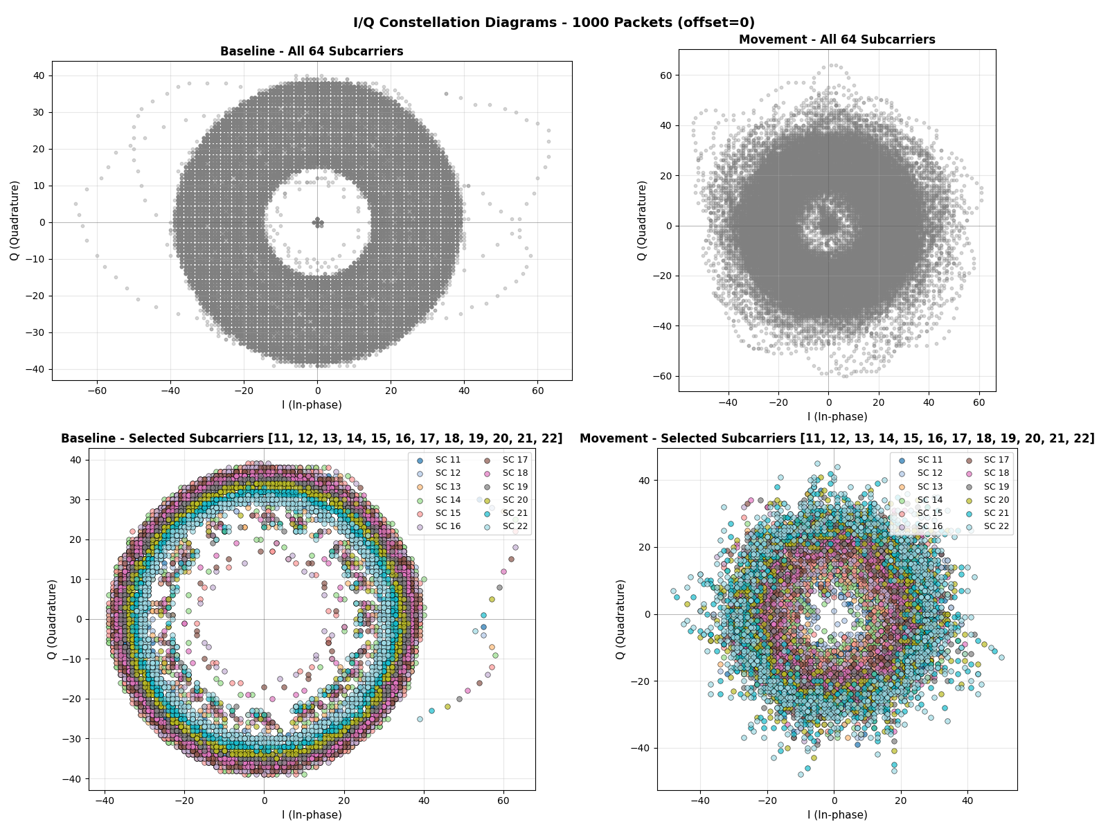I/Q constellation diagrams showing the geometric representation of WiFi signal propagation in the complex plane. The baseline (idle) state exhibits a stable, compact pattern, while movement introduces entropic dispersion as multipath reflections change.

NBVI Scoring

NBVI computes three complementary scores per subcarrier and evaluates four candidate bands derived from them. This multi-strategy approach improves robustness across different chip behaviors and RF environments.

Base score (classic NBVI):

NBVI_classic = α × (σ/μ²) + (1-α) × (σ/μ)

Where α = 0.75 by default (energy-biased weighting).

Entropy-rewarded score -- penalizes subcarriers with flat, low-information distributions:

NBVI_entropy = NBVI_classic / max(0.5, H)

Where H is the Shannon entropy of the magnitude histogram.

MAD-robust score -- replaces std with a robust estimator (median absolute deviation) to reduce sensitivity to outlier spikes:

σ_robust = MAD × 1.4826
NBVI_mad = α × (σ_robust/μ²) + (1-α) × (σ_robust/μ)

Algorithm

def nbvi_calibrate(csi_buffer, band_size=12, alpha=0.75):
    # 1. Find quietest baseline windows (P5 of variance distribution)
    windows = find_candidate_windows(csi_buffer, window_size=200, percentile=5)

    for window in windows:
        # 2. Calculate NBVI scores for all subcarriers
        for subcarrier in valid_subcarriers:
            magnitudes = extract_magnitudes(window, subcarrier)
            mean, std, mad, entropy = compute_stats(magnitudes)
            nbvi_classic[sc] = alpha * (std / mean**2) + (1-alpha) * (std / mean)
            nbvi_entropy[sc] = nbvi_classic[sc] / max(0.5, entropy)
            nbvi_mad[sc]     = alpha * (mad*1.4826 / mean**2) + (1-alpha) * (mad*1.4826 / mean)

        # 3. Noise gate: exclude subcarriers below P15 mean amplitude
        valid = noise_gate(all_metrics, percentile=15)

        # 4. Generate four candidate bands from different strategies
        band_entropy        = select_spaced(sort_by(nbvi_entropy), k=12)
        band_mad            = select_clustered(sort_by(nbvi_mad), k=12)
        band_classic_spaced = select_spaced(sort_by(nbvi_classic), k=12)
        band_classic        = select_clustered(sort_by(nbvi_classic), k=12)

        # 5. Validate each candidate with adaptive threshold (P95 × 1.1)
        for band in [band_entropy, band_mad, band_classic_spaced, band_classic]:
            fp_rate, mv_values = validate(band)
            if fp_rate <= 0.05 or fp_rate < best_fp_rate:
                best_band, best_fp_rate = band, fp_rate

    return best_band, mv_values

Selection Strategies

Two complementary strategies generate candidate bands from sorted subcarrier rankings:

Validation

Internal validation runs MVS on the full calibration buffer and calculates the false positive rate using the same adaptive threshold that will be used at runtime (P95 × 1.1):

fp_rate = count(mv > threshold) / len(mv_values)

The band with the lowest FP rate below 5% is selected. If no candidate achieves ≤5%, the one with the lowest FP overall is used.

Hint Band Logic

After selection, the calibrator optionally compares the result against a hint band (the current production default). The hint band is used only when the best candidate does not achieve ≤5% FP and the hint has a strictly better FP rate. This prevents drift to bands that minimize calibration-time FP but collapse movement recall in production.

Adaptive Threshold Calculation

After band selection, NBVI returns the moving variance values from baseline. The adaptive threshold is then calculated as a percentile with an optional multiplier:

def calculate_adaptive_threshold(mv_values, percentile, factor):
    return calculate_percentile(mv_values, percentile) * factor

See TUNING.md for configuration options (segmentation_threshold).

Why Non-Consecutive Subcarriers?

NBVI selects non-consecutive subcarriers, which provides: - Spectral diversity: Different frequency components respond differently to motion - Noise resilience: Narrowband interference typically affects adjacent subcarriers - Environment adaptation: Works well in complex multipath environments

Guard Bands and DC Zone

HT20 mode (64 subcarriers) configuration:

Default Parameters

Computational Complexity

Each candidate window generates four bands, each validated against the full calibration buffer. The dominant cost is the validation pass (O(buffer_size × band_size) per band).

Fallback Behavior

When calibration cannot find valid bands (e.g., motion during calibration, insufficient data), NBVI falls back to the default band [11-22].

See PERFORMANCE.md for detailed calibration metrics.

Signal Conditioning

Optional filters can be applied to the turbulence stream before detection. Both filters operate on the scalar turbulence value (one per CSI packet) and share the same SegmentationContext used by both MVS and ML detectors.

Hampel Filter

Enabled by default (window=7, threshold=5.0 MAD).

The Hampel filter removes statistical outliers using the Median Absolute Deviation (MAD) method, reducing false positives from sudden RF interference.

How it works:

1. Maintain a sliding window of recent turbulence values
2. Calculate the median of the window
3. Calculate MAD: MAD = median(|xᵢ - median|)
4. If |x - median| > threshold × 1.4826 × MAD, replace with median

The constant 1.4826 is the consistency constant that makes MAD a consistent estimator of standard deviation for Gaussian distributions.

def hampel_filter(value, buffer, threshold=5.0):
    buffer.append(value)

    sorted_buffer = sorted(buffer)
    median = sorted_buffer[len(buffer) // 2]

    deviations = [abs(x - median) for x in buffer]
    mad = sorted(deviations)[len(deviations) // 2]

    scaled_mad = 1.4826 * mad * threshold
    if abs(value - median) > scaled_mad:
        return median  # Replace outlier
    return value       # Keep original

Embedded optimization: Insertion sort instead of quicksort (faster for N < 15), pre-allocated buffers (no dynamic allocation), circular buffer for O(1) insertion.

Reference: [5] CSI-F: Feature Fusion Method (MDPI Sensors)

Low-Pass Filter

Disabled by default. Enable with lowpass_enabled: true.

The low-pass filter removes high-frequency noise from turbulence values using a 1st-order Butterworth IIR filter:

class LowPassFilter:
    def __init__(self, cutoff_hz=11.0, sample_rate_hz=100.0):
        wc = tan(π × cutoff / sample_rate)
        k = 1.0 + wc
        self.b0 = wc / k
        self.a1 = (wc - 1.0) / k

        self.x_prev = 0.0
        self.y_prev = 0.0

    def filter(self, x):
        y = self.b0 * x + self.b0 * self.x_prev - self.a1 * self.y_prev
        self.x_prev = x
        self.y_prev = y
        return y

Why 11 Hz cutoff? Human movement generates signal variations typically in the 0.5-10 Hz range. RF noise and interference are usually >15 Hz. The 11 Hz cutoff preserves motion signal while removing high-frequency noise.

See TUNING.md for filter configuration and tuning guidance.

MVS: Moving Variance Segmentation

The Insight

Human movement causes multipath interference in Wi-Fi signals, which manifests as: - Idle state: Stable CSI amplitudes → low turbulence variance - Motion state: Fluctuating CSI amplitudes → high turbulence variance

By monitoring the variance of turbulence over a sliding window, we can reliably detect when motion occurs.

Algorithm Steps

1. Spatial Turbulence

Computed per packet from the 12 selected subcarrier amplitudes. Uses raw std when gain is locked, or CV normalization otherwise (see CV Normalization).

1. Moving Variance (Two-Pass Algorithm) μ = Σxᵢ / n # Mean of turbulence buffer Var = Σ(xᵢ - μ)² / n # Variance (numerically stable) The two-pass algorithm avoids catastrophic cancellation that can occur with running variance on float32.

2. State Machine if state == IDLE and variance > threshold: state = MOTION elif state == MOTION and variance < threshold: state = IDLE

Performance

For detailed performance metrics, see PERFORMANCE.md.

Reference: [2] MVS segmentation: the fused CSI stream and corresponding moving variance sequence

ML: Neural Network Detector

The Insight

Motion detection can be framed as a binary classification problem: - Input: Statistical features computed from a sliding window of turbulence values - Output: Probability of motion (0.0 to 1.0)

A neural network can learn complex, non-linear patterns that may be missed by simple threshold-based methods. Unlike MVS, ML learns decision boundaries from labeled training data and generalizes across environments without per-environment calibration.

Architecture

The ML detector uses a compact Multi-Layer Perceptron (MLP):

Input (12 features)
    ↓
Dense(16, ReLU)      ← 12×16 + 16 = 208 parameters
    ↓
Dense(8, ReLU)       ← 16×8 + 8 = 136 parameters
    ↓
Dense(1, Sigmoid)    ← 8×1 + 1 = 9 parameters
    ↓
Output (probability)

Total: ~350 parameters, ~2 KB (constexpr float weights)

The 12→16→8→1 architecture was validated as optimal through architecture search on 21,665 samples (5-fold CV):

The best candidate (24-12) gains only +0.1% F1 at the cost of nearly doubling parameters and flash footprint. The 16-8 architecture offers the best balance of accuracy, size, and FP rate for embedded deployment.

Inference Pipeline

┌──────────────┐    ┌──────────────┐    ┌───────────────────┐    ┌──────────────┐
│ CSI Packet   │───▶│ Turbulence   │───▶│ Optional Filters  │───▶│ Buffer (75)  │
│              │    │ σ/μ (CV)     │    │ Hampel + LowPass  │    │              │
└──────────────┘    └──────────────┘    └───────────────────┘    └──────┬───────┘
                                                                        │
                                                                        ▼
┌──────────────┐    ┌──────────────┐    ┌──────────────┐    ┌──────────────┐
│ IDLE/MOTION  │◀───│ Threshold    │◀───│ Probability  │◀───│ 12 Features  │
│              │    │ > 0.5        │    │ [0.0-1.0]    │    │ → Neural Net │
└──────────────┘    └──────────────┘    └──────────────┘    └──────────────┘

Calibration

ML uses fixed subcarriers -- no band calibration needed:

ML uses 12 fixed subcarriers selected to avoid DC and improve stability: [12, 14, 16, 18, 20, 24, 28, 36, 40, 44, 48, 52]. This eliminates the 7.5-second band calibration phase, reducing boot time to ~3 seconds (gain lock only).

Features

The ML detector extracts 12 non-redundant statistical features from a sliding window of 75 turbulence values (configured via segmentation_window_size).

Design principles: - No redundant features (e.g., no variance alongside std, no range alongside max/min) - 12 turbulence-window features (11 statistical + 1 temporal-variation) - MicroPython compatible: pure Python implementation without numpy at runtime

Feature Categories

Basic Statistics (0-3): Standard statistical measures of the turbulence buffer.

Signal Dynamics (4): - Zero-crossing rate: Fraction of consecutive samples crossing the mean. High ZCR indicates rapid oscillations (motion), low ZCR indicates stable signal (idle).

Higher-Order Moments (5-6): Computed from the turbulence buffer (75 samples) for stable estimates. - Skewness: Asymmetry of turbulence distribution. Motion typically increases skewness. - Kurtosis: "Tailedness" of turbulence distribution. Motion produces heavier tails.

Robust Statistics (7, 9): - Entropy: High during motion (unpredictable), low during idle (stable) - MAD: Robust alternative to std, less sensitive to outliers

Temporal Structure (8, 10): - Autocorrelation: Lag-1 temporal correlation. High during idle (smooth signal), low during motion (turbulent) - Slope: Positive = increasing turbulence, negative = decreasing

Temporal Variation (11): - Waveform Length: Sum of absolute first differences over the turbulence window. Higher values indicate faster/more irregular short-term motion dynamics.

Feature Importance

SHAP and correlation can diverge significantly: correlation captures linear association with the label, while SHAP captures non-linear contribution inside the network.

Updated values from 10_train_ml_model.py (--correlation and --shap):

Feature Definitions

Zero-Crossing Rate:

ZCR = count(sign(x[i] - μ) ≠ sign(x[i-1] - μ)) / (n - 1)

Counts how often the signal crosses the mean value. Ranges from 0.0 (monotonic) to 1.0 (alternating every sample).

Skewness (third standardized moment):

γ₁ = E[(X - μ)³] / σ³

• γ₁ > 0: Right-skewed (tail on right)
• γ₁ < 0: Left-skewed (tail on left)
• γ₁ = 0: Symmetric

Kurtosis (fourth standardized moment, excess):

γ₂ = E[(X - μ)⁴] / σ⁴ - 3

• γ₂ > 0: Heavy tails (leptokurtic)
• γ₂ < 0: Light tails (platykurtic)
• γ₂ = 0: Normal distribution (mesokurtic)

Shannon Entropy:

H = -Σ pᵢ × log₂(pᵢ)

Computed by binning turbulence values (10 bins) and calculating the entropy of the histogram. Higher entropy indicates more randomness/unpredictability.

Lag-1 Autocorrelation:

r₁ = (1/(n-1)) Σ(xᵢ - μ)(xᵢ₊₁ - μ) / σ²

Measures temporal correlation between consecutive values. Ranges from -1.0 to 1.0. Smooth signals have high positive autocorrelation; turbulent signals have low autocorrelation.

Median Absolute Deviation:

MAD = median(|xᵢ - median(x)|)

Robust measure of spread. Unlike std, a single outlier cannot dramatically inflate the MAD. Computed using insertion sort (efficient for n=75 on ESP32).

Linear Regression Slope:

slope = Σ(iᵢ - ī)(xᵢ - x̄) / Σ(iᵢ - ī)²

Where i = time index, x = turbulence value. Positive slope indicates increasing motion intensity.

Waveform Length:

WL = Σ |xᵢ - xᵢ₋₁|,  i = 1..n-1

Measures total temporal variation in the turbulence window. Compared to slope/autocorrelation, it is more sensitive to short, bursty oscillations and does not require logarithms or histogram binning.

Training

For the complete training workflow (data collection, training commands, export formats), see ML_DATA_COLLECTION.md.

The training pipeline includes:

• Chip-grouped cross-validation: Uses StratifiedGroupKFold with chip type as group, so each fold's validation set contains chips not seen during training for that fold. This prevents inflated CV metrics from chip-level data leakage and ensures worst-chip recall is tracked during development.
• Hard-positive sample weighting: Movement samples near the MVS detection threshold (subtle motion) receive higher training weight, while easy positives receive lower weight. This focuses the model on the boundary cases where recall drops in deployment.
• Stratified validation split: The internal early-stopping validation set uses explicit stratified splitting rather than Keras's default sequential split, preventing chip imbalance in the validation data.
• Early stopping and LR scheduling: Patience-based early stopping with best-weight restoration and reduce-on-plateau learning rate scheduler.
• Dropout regularization: Applied between hidden layers during training (automatically disabled at inference).

Performance

ML achieves higher recall than MVS with a small tradeoff in precision. ML's strength is generalization -- it performs well across different environments without per-environment calibration.

See PERFORMANCE.md for detailed per-chip results and TUNING.md for configuration and tuning guidance.

References

1. Subcarrier selection for efficient CSI-based indoor localization (2018)
   Spectral de-correlation and feature diversity.
   Read paper

2. Indoor Motion Detection Using Wi-Fi Channel State Information in Flat Floor Environments Versus in Staircase Environments (2018) Moving variance segmentation.
   Read paper

3. WiFi Motion Detection: A Study into Efficacy and Classification (2019) Signal processing methods for motion detection.
   Read paper

4. A Novel Passive Indoor Localization Method by Fusion CSI Amplitude and Phase Information (2019) SNR considerations and noise gate strategies.
   Read paper

5. CSI-F: A Human Motion Recognition Method Based on Channel-State-Information Signal Feature Fusion (2024) Hampel filter and statistical robustness.
   Read paper

6. Linear-Complexity Subcarrier Selection Strategy for Fast Preprocessing of CSI in Passive Wi-Fi Sensing Classification Tasks (2025) Computational efficiency for embedded systems.
   Read paper

7. CIRSense: Rethinking WiFi Sensing with Channel Impulse Response (2025)
   SSNR (Sensing Signal-to-Noise Ratio) optimization.
   Read paper

License

GPLv3 - See LICENSE for details.